Frequently Asked Questions
The Time Series functionality moved locations in DNS v6. It can now be found under the Global Settings button in the Configuration tab (see image below).

To export .doric files as .csv you should use the Doric File Editor module (see images attached). Briefly, by loading all your .doric data files within the Doric File Editor plugging (find under Analysis option in the Menu in Doric Neuroscienc Studio), you can click the ‘Export’ icon to save them as CSV files. However, this function can only export one channel at a time.
Note: if you are using Matlab, Python or Octave, you can directly read .doric files with code provided here. With a small modification to your data analysis pipeline (a few lines of code at most), you can easily replace .csv file with .doric file. The advantage of the .doric file (HBF5-based) is that it saves both the raw data and the recording parameters together (useful for troubleshooting and/or reproducibility). We’ve moved to this file format in version 6 because it can handle metadata (behavior videos, images, signal, TTL, etc.) and stores very large data efficiently.

Doric Neuroscience Studio (DNS) is an intuitive software that controls Doric hardware beside recording and analyzing optogenetics, fiber photometry, electrophysiology, and behavior camera data.
Any other behavior data (for instance pressing a key in the arena) that is obtained in voltages using a BNC cable (maximum 10 V) can be recorded by the Doric console either via DIO ports (if the data is on/off mode) or AIN port (for sinusoidal data) simultaneous with the photometry recording and be aligned in time. Above this voltage an extra adaptor is required to adjust the voltage level.
All information coming to console and then DNS will be saved as a single file with .Doric format, containing subfolders for each channel, and they can be loaded and analyzed all together later.
DNS software can livestream the data collection for all channels simultaneously.
The software also contains the following data analysis modules:
- Signal Analysis module (fiber photometry ΔF/F, filters, arithmetics, spike finding, ...)
- Behavior Analysis module (open-field tracking, motion score, and speed)
The negative signals in the image below are what we call ‘packet-loss artifacts’. These types of artifacts can occur when data points are lost during data acquisition.

Troubleshooting packet-loss artifacts:
Set the software to high-priority, as in DNS-priority.png. (This makes Windows prioritize Doric Neuroscience Studio over any operations running in the background that can tax the computer.)

Double-check that the console is directly connected to the computer via a USB 3.0 or USB SS (superspeed) port. USB 2.0 ports on the computer are also too slow and often lead to data loss.
Do not use USB Hub (even if it is USB 3.0). Most off-the-shelf USB hubs do not have the bandwidth and/or speed to properly transfer data from the console to the computer without loss. If required, we sell USB hubs that are thoroughly tested with our equipment (or you can re-arrange USB connections so that the console is directly connected to USB 3.0 of the computer.)
Avoid: recording data using Remote Access or Zoom or other taxing software when recording data; Remote Access in particular leads to poor data quality and many pack-loss artifacts.
In the new versions of DNS (starting from v 6.4.2.0), we added an image lost counter at the bottom of the microscope view and replace the dropped frame by a copy of the previous one. The number of dropped frame and their timestamp are also saved in an attribute of the dataset:


DNS v6 saves data into an HDF5 file with the ".doric" extension.
Files saved with DNS v6 can be analyzed with its data analyzer modules, but the HDF5 files can be read with other applications as Matlab, R or Python.
We created a GitHub repository with code examples to facilitate data analysis with external applications : Github![]()
You have a few different options to analyze data in the .doric format:
-
We recently came out with danse™ which is a software designed to analyze .doric files. Specifically, with NO coding required, danse™ can:
-
Basic processing (remove artifacts, decimate, linear interpolation, calculate dF/F0, find spikes, etc.)
-
Import stimuli/behavior events and behavior videos from other devices
-
Calculate behavior events that are time-locked to the neural activity (including Animal tracking, calculate animal presence in zones, animal distance from points, Motion score, and create behavior events from all those behavior measures using adjustable threshold)
-
Create plots that combine neural activity and behavior data (e.g. peri-event/ peri-stimuli time histograms)
-
Automatize data processing and data analysis pipelines without coding required
NOTE: The Technical Support Tab of our website now contains many danse™ tutorial videos which can give you an idea of what the software can do. Currently, only photometry-related content has been made in tutorial form, but we are consistently adding to this video library with behavior and microscopy tutorial videos coming soon. If you are interested in this option, contact us at sales@doriclenses.com for a free 15-day trial and/or a quote. We also provide virtual demos through zoom, including a walk-through using your own data with us to see how you can best utilise the software to analyze your specific experiments.
-
Doric Neuroscience Studio (DNS), our free data acquisition software, contains the Signal Analyzer, Image Analyzer, and Behavior Analyzer modules which include some basic data processing tools that are also offered by danse™ (like calculating dF/F, find spikes, etc.).
-
If you are interested in using Matlab, Python, R, or Octave, you can directly read .doric files with code provided on our GitHub repository. This includes the .doric output of the Signal Analyzer, Image Analyzer, and Behavior Analyzer modules. This allows you to do further analyses on Photometry dF/F0 calculations to create your plots and calculate your stats in either of those softwares.

Here are instructions showing how to use 405 nm (isosbestic signal) to remove motion artifacts from a red signal in danse:
- Decimate signal (not necessary if using default Lock-In settings in DNS, which automatically decimate by 200x).
- Baseline Correction (remove exponential decay due to photobleaching to flatten the signal).
- Align signals (this standardizes isosbestic and biosensor signal so that they can be properly subtracted)
- Subtract isosbestic from biosensor signal
- Filter the signal to remove high-frequency noise (optional)
See example of this is correction, which successful calculated dFF for red signal and remove of motion artifacts.

See the example of pipeline and parameters used in danse™ software to correct the above example:


Instruction for using Statistic Analysis:
- Calculate photometry signal dF/F: Check this video for more information.
- Find Spikes: Check this video for more information.
- Note video does not include updated features like interation (which allows the identification of smaller spike when there are very big spikes present in the recording) - Create TimePoints (as in image1). Note that the timepoints must be in seconds (not minutes).
- Select Analysis button (like for PeriEvent), but instead of selecting the Analysis = PeriEvent, select Statistics
- Then choose spikes as the signal (like image2)
- Then select Timeperiods and what analysis you would like between spike amplitude, spike frequency or spike count (as in image3)
Note that the Statistic operation can also be used for Events instead of timeperiods.
Image1:

Image2:
Image3:

Here are the instructions:
- Calibrate the video (set pixel-to-dimension conversion factor for proper speed measurements).
- Draw Area
- Animal Tracking (Body)
- Update Animal Tracking Coordinates (if needed, for example, to label nose to more easily identify interactions)
- Draw Zones and or distance from points
- Computer Prescence in Zone / Distance from points
- Create Events from Prescence in Zone / Distance from points (see image)

The goal of Lambda parameter is to remove the exponential decay (slope of the entire recording) of the photometry signal that arises due to photobleaching and obtain a nice flat DF/F trace. The lambda value is used to find the shape of this slope. Ideally, the displayed fitting line should nicely trace this exponential decay without picking up small fluctuations (and especially do not pick up real peaks in the data), as it will remove real signal!)
This link provides a general comparison among all Doric photometry products. Also a useful guide presenting and comparing our different photometry systems may be found here. This guide, in addition to going through their specificities, may also guide you towards a system that may better fit your own experiment. If you need further assistance with this, contact one of our specialists at sales@doriclenses.com.
The Technical Support Tab of our website now contains several tutorial videos providing some help with photometry systems installation and set-up. If you need further assistance with setting-up your system, contact one of our specialists at sales@doriclenses.com.
If you are using a standard basic fiber photometry setup read information below:
In general, the standard fiber photometry consists of multiple pieces including: computer interface, console, LED driver, light source, mini-cube, detector, fiber and cannula. A diagram below shows the interconnection of these components.
All commands initiated in the software first reach to the console. Console is typically the control hub of the system, managing all the connections. The console is equipped with three types of ports: the analog output (AOUT), analog input (AIN) and digital input-output (DIO). Upon receiving software commands, the console converts them into voltages and transmits them to the LED drivers through the AOUT ports. The driver then converts voltages into preset current intensities to trigger LED light excitation. Depending on these current, the light sources (LEDs or lasers) will generate the excitation light spectrum. The excitation light then passes through filters and dichroic mirrors inside a cube and reaches to the tissue by optical fibers. The fiber and cube also return the collected neuronal fluorescence emission to the detector which converts light intensities into currents and amplifies them. Those currents are finally sent back to the console via AIN ports.
Remarkably, as mentioned before the console also contains DIO port that are useful for connecting external devices such as an optogenetics system, camera or even a second photometry system, …. DIO ports in this case are useful for synchronizing the additional devices with the photometry system.

We usually recommend using the Lock-In mode over the interleave mode for our basic photometry system, as it provides several advantages (see below). Note that if you need to record isosbestic, green photometry and red photometry, you have to use Lock-In mode, as the FPC console’s interleave mode can only handle interleaving two signals (and not three). In addition, for most systems, the isosbestic and GCaMP signal are sent to the same detector, and split using the demodulation or deinterleave algorithms (see more details on this process in the explanation below).
The two modes are related to the two different ways to separate light arising from the sample into different signals (isosbestic, green and red photometry):
(1) frequency-division (Lockin)
(2) time-division (interleaved)
LockIn mode: frequency division
In this mode, all LED excitations are turned ON during the entire duration of the recording. However, they are oscillating between a minimum and maximum power at different preset reference frequencies (e.g. 208.616 Hz, 166.893 Hz, etc.) that we’ve carefully chosen. Notice that the sampling rate is a higher range than the when using interleaved mode.


The raw signal (c) collected by each detector is a summation of many frequencies (fluorescence in response to 405 excitation, fluorescence in response to 465 excitation, ambient light, electrical noise, autofluorescence of the tissue and patch cord, etc.). We use a demodulation algorithm to mathematically separate the fluorescent signal oscillating according to each reference frequencies (these are the demodulated traces, LockIn-AIN01xAOUT01, etc.). This is useful as it removes noise occurring at different frequencies and makes the signal invariant to ambient light (as ambient light flickers around 60Hz).
* For a full tutorial on how to set-up the configuration based on the wiring of your system see this video.
Interleaved mode: time division
In contrast, in the interleaved mode, only one LED is turned on at a time at a defined frequency (choose between 10-100 Hz). We have a live de-interleaved algorithm that splits the fluorescent signal corresponding to the time only the 405 led was on and the time only the 465nm LED was on. One thing to be careful is that tuning on and off the LED create small electrical artifact that adds noise to the signal. In addition, the interleave mode does NOT ignore different frequencies of light, so it is not invariant to ambient light. The last limitation of this mode is that (for the FPC console) it only support interleaving two signals (but the NC500, our newer console can interleave up to 4 signals).

Comparison between interleaved and LockIn modes:
|
Interleaved mode |
LockIn mode |
|
|
Maximal Temporal Frequency |
60 Hz |
1000 Hz |
|
Compatible Photometry Systems |
Basic & Bundle |
Basic only |
|
Number of signals |
2 (basic) up to 3 (bundle) |
Up to 4 |
|
Sensitive to ambient light |
YES |
NO |
No signal: (dips and bumps are almost identical between experimental and isosbestic trace)

Weak signal (bumps in the functional signal do not occur in the isosbestic trace but low in amplitude)

Strong signal (bumps in the functional signal do not occur in the isosbestic trace)

Depending on the system, the expression level of the recorded fluorophores, and a bunch of external factors, these values will always be different and must be optimized for your specific conditions. A good starting point is to look up papers in the brain region of interest and/or that used your fluorophore. The LED power is usually reported and can give you an idea of a more specific range of power for your case. We do recommend though that the isosbestic power be half the power of the experimental signal. This will reduce photobleaching. You should measure the LED power of each LED one at a time (turn off LEDs in the LED Driver module).
There are two possibilities: either settings are not optimal or there is a malfunctioning component within the system.
-
For FMC or iFMC systems (with external LEDs)
-
Check the connections of the system. In particular, ensure the Connector keys are well aligned in the receptacle slots, especially when tightening the coupling nut (see image below). Misalignment can significantly reduce transmission through the fiber and lead to sever drops in power.

-
Set the LED Driver in CW mode, and low-power mode with max current (200 mA) to reproduce the minimum and maximum power figures given on the LED and iFMC datasheet. If they differ more than 10%, contact Doric support (support@doriclenses.com) to ensure the device is working properly.
-
ilFMC Gen.2 systems (with integrated LEDs, but separate LED Driver)
-
Turn adjustment ring (silver ring) clockwise to increase transmitted power through the variable attenuator (see image below)
-
Check the connections of the systems. In particular, ensure the Connector keys are well aligned in the receptacle slots, especially when tightening the coupling nut (see image below). Misalignment can significantly reduce transmission through the fiber and lead to sever drops in power.
-
Use a power meter and a 400µm NA0.57 patch cord with the current set to 200mA to reproduce the minimum and maximum power figures given on the ilFMC datasheet. If they differ more than 10%, contact Doric support (support@doriclenses.com) to ensure the device is working properly.

-
ilFMC Gen.3 systems (with integrated LEDs and LED Driver)
-
Check the connections of the systems
-
Use a power meter and a 400µm NA0.57 patch cord with the current set to 500mA to reproduce the maximum power figure given on the ilFMC datasheet. If they differ more than 10%, contact Doric support (support@doriclenses.com) to ensure the ilFMC is working properly.
Since ~80% of the photometry signal arises from the volume of tissue located at a depth of ~200 μm from the facet of the fiber, the approximate area of FOV for each core diameter is directly related to the diameter of the patch cord. (You simply can calculate the area of each patch cord using diameter to see the difference in FOV.) The NA of the patch cord will change the shape and depth of the data collections. You can learn more about the effect of the core diameter and NA on photometry data collection in this paper. Note that people use different diameter patch cords depending on the size of their region of interest. If your region of interest has a diameter of around 200um, use the 200um patch cord. If it's larger, use the 400µm core instead. You will get 75% more signal using a 400µm core since you can image many more neurons with this larger area patch cord. For fiber photometry larger NA is recommended to collect more signal; While it is true that a lower NA will increase the penetration depth, when we recommend a high NA fiber, we assume that the cannula is placed close (less than a few µm) to the detection area. Then, since the position can be manually optimized, we recommend optimizing the fluorescence collection with a high NA fiber.
-
One of the causes of movement artifact on the signal is the optical transmission of the rotary joint that may vary in rotation.
-
If the rat generates fast acceleration, it can be difficult to correct those motion artifacts.
-
The system embedded on the rotor of a torque-assisted electrical rotary joint, as the RFMC or the RBFMC, will remove those signal variations, as the sensor is on the rotor directly, then does not pass through an optical rotary joint.
-
Other causes of movement artifact are the fiber bending losses and the movement of the fiber implant. The fiber bending loss is difficult to prevent. You may consider using a stronger jacket, i.e. ARMO jacket instead of the 1.1 mm hytrel jacket for the patch cords to the animal. It is less flexible, and will affect more the behavior, but is acceptable for rats. And it will help the cable to survive longer.
-
Movement of the fiber implant requires good cementing and maybe protection around the implant to make sure it is stable. For mice, it is less of an issue, but for rats, we know that researchers add some features to solidify the implant. You may consider using the 2.5 mm ferrule instead of 1.25 mm, or another type of receptacle. You may take a look here for more detailed information regarding the implants we offer.
Minicubes with integrated LEDs reduce the number of optical connections and the system's overall footprint, which overall simplifies the system. However, it offers less flexibility to the user in terms of the light sources to be used. On the other hand, non-integrated minicubes present larger number of components and space, but modularity increases flexibility so that you can use different LEDs / lasers and/or fluorophores in the future than by replacing a few components required instead of buying a whole new system.
NOTE: there is no price difference between an integrated mini cube and a non-integrated mini cube with LEDs and cables purchased separately.
While the isosbestic point of GCaMP fluorophores have been well characterized and 405 and 415nm being widely used in green photometry, red photometry is still in its infancy. There are some who do not use an isosbestic point at all for either color of photometry (even though it is a nice way to control for background fluorescence/artifacts, especially in freely moving animals).
We usually recommend using the DC mode. When in DC mode, the signal from the photodiode is directly passed along to the amplifier without alteration. The output range at the BNC connector is 0V to 5V. This mode is recommended for photometry experiments and should be used by default unless specified otherwise. When in AC mode, the signal from the photodiode is passed through a 30Hz high-pass filter before going to the amplifier. Any variations lower than 30 oscillations per second as well as the average value of the signal is removed. The output range at the BNC connector is -5V to 5V. This mode offers twice the dynamic range but can hide a state of saturation of the pre-amplifier and should be used with care.
The gain switch selects between three or two (depending on mini-cube generations) output level for the same input fluorescence light. The 1x gain passes the signal from the pre-amplifier directly to the BNC while the 10x and 100x add 2 other amplification levels. Gain selection should be done only for very coarse signal adjustment. Gain should be lowered if the amplifier is saturated (at line around 5V) and increased if is lower than 0.5V. It is quite common that the 10X amplification is used for photometry experiments, but this will also depend on your signal.
-
FRJ_1x1_PT: 2% peak-to-peak
-
FRJ_2x2_PT: 3% peak-to-peak
-
AFRJ_2x2_PT: 3% peak-to-peak
The Isosbestic point is the excitation wavelength at which the fluorescence intensity of the bound and unbound states are equal and do not dependent on the relative concentration of each state.
To simplify it lets focus on GCaMP calcium indicator (Fig. below). GCaMP, like other genetically encoded calcium indicators has a fluorescence property. Meaning that when exposed to a specific light wavelength (excitation light, blue traces), it emits light at a longer wavelength (emission light, green traces). However, when Ca2+ ions bind to GCaMP, it undergoes conformational changes that increases its fluorescence property. Therefore, the light spectrum that induces emission is a bit different for the bound (solid line in Fig.) and unbound (dashed line in Fig.) states of GCaMP. However, as shown below, the fluorescent intensity traces for the two-forms of GCaMP cross (are equal) if the excitation light is applied around 405 nm (red dot in Fig.), therefore both bound and unbound GCaMP proteins fluoresce at similar intensities, which resembles the baseline level.
In photometry experiments, recording a precise isosbestic baseline can serve multiple advantages.
For instance, GCaMP Ca2+-dependent signal can be contaminated by the movement artifacts, autofluorescence, and photobleaching. Those contaminations will distinctly appear in the isosbestic baseline trace as well and can be used in post-processing to remove them from the GCaMP Ca2+-dependent signal. Thus, the goal of isosbestic signal is to provide a control or reference signal to distinguish true peaks from artifacts.
*Please note the isosbestic range varies for different genetically encoded calcium indicators, therefore it needs to be chosen with precision.

Following references list the isosbestic point for frequently used calcium indicators:
Eleanor H.S et al. Lights, fiber, action! A primer on in vivo fiber photometry. Neuron Mar 6; 112(5): 718–739 (2024).
Hod D. et al. High-performance calcium sensors for imaging activity in neuronal populations and microcompartments. Nature Methods Jul;16(7):649-657 (2019). (See supplementary)
Rosana S.M et al. Understanding the Fluorescence Change in Red Genetically Encoded Calcium Ion Indicators. Biophysical Journal May 21;116(10):1873-1886 (2019).
Cody A.S et al. Leveraging calcium imaging to illuminate circuit dysfunction in addiction. Alcohol. Feb; 74: 47–63 (2019).
In fiber photometry, saturation occurs when the intensity of the emitted light from the sample surpasses the capacity of the detector. In such cases, any further increases in the emission light (such as a calcium peak) will not be detect, as the detector has already reached the maximum value.
The images below show an example of a saturated signal at two zoom levels.


To properly be warned of signal saturation, make sure to specify the right detector type in the Doric Neuroscience Studio (DNS), as different detectors will saturate at different maximum voltages (e.g. Doric = 5 V, while Newport = 7.5 V). Specifically, in the Analog Input setter, set the Saturation parameter to the appropriate detector name. The saturation level is a feature defined by detector hardware and it cannot be modified.

Signal saturation can stem from various factors:
1. Too much light going into the tissue, either:
a) Ambient light from the environment is reaching the detector.
b) Excitation Power is too high.
2. Too much fluorescence going to the detector:
a) Amplification/Gain setting is too high
b) Strong fluorophore expression
We will see the solution to each factor:
1a: Ambient light can reach the recording site when researchers use transparent cement for their implantations. Instead, we recommend dying dental cement black to block ambient light penetration. Some people will even color the dental cement with black sharpy or black nail polish. Alternatively, if the experiment permits, you can also record in the dark or near dark.
1b: see reducing LED power instructions
2b: Strong fluorophore expression:
- Reduce LED excitation power. (See instructions for that.)
- Make sure to not overexpress the fluorophores (GCaMP, G-GECO, etc.) in the region of interest. Avoid using very high volumes of viral construct injections and consider using a lower titer of viruses.
If the saturation remains during recording, you can use two solutions:
In the DNS software, use low-power mode and reduce the value of LED Power %.

2a: Reduce the detector Gain/Amplification. For the majority of photometry experiments, the gain should be 10x when the system is connected to the animal.
- If the gain is at 100x: reduce it to 10x.
- If the gain is already at 10x:
- Reduce LED excitation power (see solution 1b)
- If reducing the power did not solve the saturation: reduce gain to 1x.
Photobleaching is among the commonly observed issues during fiber photometry, as a steep drop in photometry signal intensity during the first few seconds of recordings. This decrease is caused by various factors including the light-induced patch cord bleaching, fluorescent reporters, and autofluorescence from the tissue itself.

Signal disappearing due to photobleaching
In some cases, the fluorescent molecules irreversibly lose their fluorescence emission property. This can occur especially if molecules are exposed to high intensity or long duration of excitation light. In this case, signals detected during the first recording may be gone the following day. In such a case, waiting a 1-2 week for the tissue to replenish fluorophore AND reducing excitation power usually solves the issue.
To reduce the effect of patch cord bleaching and reduce background fluorescence in the signal, it is recommended to bleach the patch cords once per week. To do so, set LED to CW mode at maximum current/voltage for a minimum of 1 hour, but ideally overnight. Here is a document detailing the recommended Patch Cord bleaching protocol. Note that you can create a designated software configuration with high power settings to bleach overnight.
To reduce photobleaching during photometry recordings, it is recommended to keep the patch cord power among 10-60 µW. Note that there is always a trade-off between signal strength and photobleaching.
Post-processing correction of photobleaching
The exponential decrease in the photometry signal is usually corrected in post-processing using Baseline Correction Algorithms (like the ones offered in DNS Signal Analyzer and Danse™).
Before correction

After Correction

When combining blue optogenetic stimulation with red photometry usually researchers report huge artifacts appearing in their recordings (image 1 below). In fact, blue light naturally causes autofluorescence from the silica inside the patch cord at red spectrum (reference, Figure 7b). This artifact is proportional to the blue excitation power used. So, a first potential solution would be to decrease the power of your optogenetic excitation.
If you are using a frequency-division (Lock-In mode) strategy for photometry and TTL pulses (square pulses) for optogenetics stimulation this does not work well with the algorithm and every time the laser opto-stim is turned on or off, it will increase the baseline noise. Instead, you can try using analog signals (sine waves instead of square pulses, at the same frequency), as analog signals work better with the demodulation algorithm.
In addition, check whether you are saturating the red detector. Blue optogenetic light is usually much stronger than blue photometry excitations (mW vs uW). Saturation of the detector will prevent detection of any peaks, as the detector is already at maximum.
Possible Solutions:
1. Reducing blue excitation power.
2. Instead of using square pulses for your optogenetic excitation, try converting it to an analog signal with sine waves.
3. Check that you are not saturating any detectors. (If you are saturating the detector, then you should again reduce opto excitation power.)
4. Use Interleave mode instead of the Lock-In mode (time-division instead of frequency-division), such that your optogenetic excitation and photometry recording are never at the same time (image 2 below).
5. Change your experiment design: use red opsin with green photometry instead.
Image1:

Image 2:

In fact, green fluorophores, commonly have excitation (E) peak at 490 nm. However, as their fluorescent emission (F) is very close to E range, it is an industry-standard to excite slightly off-peak and then maximize the detector filter to obtain a better signal. This range has the added benefit of avoiding the tail-end excitation of the red biosensors.
The excitation and emission filters are predesigned inside the cubes and cannot be modified. As so, using an LED with a peak excitation (490 nm) that is not matching the cube filter peak range (475 nm), might lead to weak excitation power. Plus, the 490 nm LED has relatively less power intensity compared to the 475 nm LED, therefore overall, the power will be lower. This can probably be adjusted using lower attenuating patch cord to compensate and keep the power of excitation high enough.
Besides centering the excitation filter around 490 nm excitation can lead to crosstalk with emission spectrum inside the cube.
The image below is an example for GCaMP6f, comparing two different conditions for E and F ranges. To prevent the excitation light from being picked up by the detector (cross-talks), we need a minimum distance between E and F for 10 nm. So, the more the excitation is shifted to the right (second image), the more the detector filter range will have to also shift to the right, which can lead to significant signal loss (see red arrow). As shown in the second image area under the curve (AUC) is smaller for F detection, meaning that the photometry signal will be weaker.
* Image from https://www.fpbase.org/

This paper reported the isosbestic range of a large number of sensors. It is shown that not every sensor has an isosbestic point. One alternative is to use a non-dynamic fluorophore as a control (like tdTomato), instead of the isosbestic point. You can read more about this option in the same paper above.
The new Doric photometry system comes with additional choices of isosbestic points: 350, 405, 415, 425, 430, 440 nm, etc. We also offer a custom ‘flexible isosbestic’ option, for new photometry systems compatible for diverse set of biosensors. Both of these options require special filters inside the cube that support multiple isosbestic points (so it cannot be retrofitted for older photometry systems).
Regardless, some people have published using 405nm isosbestic as a control signal even, if it is not the true isosbestic point of their sensor (this is quite common for dopamine sensors in the literature). However, it requires further investigation to make sure it is still valid to say that peaks common to red and isosbestic are not real signals, especially when correcting for motion artifacts.
That being said, if 405 is not the true isosbestic signal, care should be taken so that subtraction does not cause artifacts or artificially amplify the signal. This is especially crucial if the signal is quite strong, as very strong signal will lead to measurable ‘downpeaks’ in the isosbestic basically mirroring the biosensor signal (see image below). If this occurs, we recommend reducing the excitation power to minimize ‘mirroring effect’ of isosbestic as much as possible.

For microscopes using an USB-3 connection to the computer (eTOSM, eTSM-Gen3):
-
Ensure that the Microscope Driver is plugged into the computer using the provided USB-3 cable.
-
Ensure that the Electrical Cable Connector is plugged into the appropriate device (computer and microscope).
-
When the 1-color Microscope Driver is activated, the On/Off Switch should be on ON and the white LED blink while initializing. If the light is sustained without any blinking when first turned on, restart the Microscope Driver.
For microscopes using an ethernet connection to the computer (SFM, 2CFM):
-
Ensure that the Microscope Driver is plugged into the computer using an Ethernet cable.
-
Ensure that the Electrical Cable Connector is plugged into the appropriate device. The Microscope Driver must be linked to the Microscope.
-
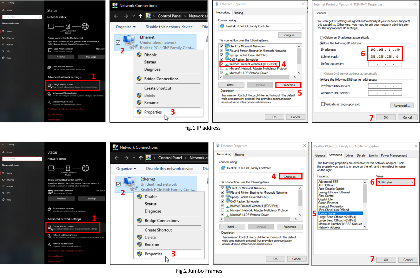
Ensure that the IP address is static (see Fig.1)
-
Ensure the Jumbo Frames are activated (see Fig.2)
-
Windows Firewall can prevent communication. To ensure the communication is not being blocked, open the Windows Firewall configuration window, then click on Allow an app through the firewall. From there, select the Change Settings button, find Doric Neuroscience Studio software and check the Private and Public checkboxes.
-
In the Network & Sharing Center, check the Ethernet connection; it should indicate Unidentified Network. If Network Cable Unplugged is shown despite the Ethernet cable being plugged in and the driver being turned on, disable and re-enable the Ethernet connection.
-
Ensure Network & sharing is properly configured at 1 Gbps by double-clicking the Ethernet connection and checking the Speed.
-
When the 1-color Microscope Driver is activated, the On/Off Switch should blink blue while initializing. If the light is sustained without any blinking when first turned on, restart the Microscope Driver.
If you need further assistance with this, contact one of our specialists at support@doriclenses.com.
The microscope driver must be connected to a computer ethernet port. Should a USB to Ethernet adapter be used for other function, such as internet access, the adapter must be disabled during the first initialization of the microscope.
While running a microscopy experiment with Doric Neuroscience Studio, we recommend deactivating all internet-using programs that can conflict with the Doric Neuroscience Studio (i.e Skype, Firewall, etc.)
In addition, we recommend using a computer with these specifications:
-
Operating System: Windows 10 or 11
-
CPU: Quad Core I7 3.46 GHz
-
RAM: 16 Gb
-
Dedicated Graphics Card: with Open GL version 4.6 recommended
-
Desktop computer recommended
Finally, Windows might limit the performances to reduce energy consumption.
To ensure that the communication is not limited, open the Power option window and follow these steps:
-
Press the Windows + R keys to open the Run dialog box.
-
Type in the following text: “powercfg.cpl”, and then press Enter.
-
In the Power Options window, under Select a power plan, choose High Performance.
-
If you do not see the High Performance option, click the down arrow next to Show additional plans.
-
If available, change the System standby and System hibernates settings to Never.
-
Click Save changes or click OK.
*Dropped frames are black frames that occur when an image is lost in communication. They can easily be spotted in the Average Intensity in ROI trace if the value descends to 0.
The images obtained with Doric Neuroscience Studio are saved in a .doric format, which is a HDF5 type format. They can be visualized using softwares supporting HDF5 format such as Doric Neuroscience Studio (using the Image Analyzer plugin), ImageJ (Import function and various plugins) or a HDF viewer. Code examples are also provided here on our website and allow to read the images in Python, Matlab and Octave.
We recommend that the optical fiber Patch Cord is of equal or shorter length than the microscope Electrical Cable when connected to the Assisted Opto-Electric Rotary Joint. Even if the cable is looped, the distance from rotary joint to patch-cord connector should be shorter than the length of the electrical cable.
These two components are meant to be glued together after installation. If they have not been glued during installation, add a drop of quick-drying glue on the border between the Cannula and Protrusion Adjustment Ring.
Fill the interior of the Cannula with KWIK-CAST (WPI) to act as a cap. After removal of the dried sealant, clean the Rod Lens outer surface using a cotton swab lightly dipped in isopropyl alcohol.
- Ensure that the Microscope Clamps are sufficiently loose (screw in the barrel).
- Ensure that the Cannula and Microscope Body are properly aligned.
- Verify the Cannula installation instructions . Some tips are available in this application note. You may also have a look at this one-color microscope instructional video or this video for two color microscope.
-
We recommend first ensuring that the microscope body is correctly connected to the implant baseplate, since a small gap between both may affect signal transmission and/or illumination.
-
Usually, the system can distinguish cells 2 or 3 weeks after the implantation of the cannula. Nonetheless, better image quality is obtained 2-8 weeks after the implantation. The waiting time for tissue repair can be a good period to use the Dummy Microscope to train the animal tolerating the encumbrance of a microscope on its head and to get used to moving easily in its cage with it. If you are imaging 2-3 following implantation, consider waiting another 10 days-2 weeks before trying again. If the issue persists, consider checking implant positioning in the sample towards the location of the fluorescent cells to image (to check whether they are out of range from microscope working distance)
In the latest version of Doric Neuroscience Studio v5, a new file format, .doric format, was introduced, and this format is the sole format to be saved in the latest v6 versions. Data is exclusively saved in HDF5 files .doric extension format (.csv and .tiff format from version 5 are no longer available). HDF 5 files can be read with Matlab, Octave, and Python. Code examples are provided to facilitate data analysis with those external applications.
The use of .doric file format over other formats provides several advantages:
-
Stores heterogeneous data types (such as signal vectors, images,and videos) in a single file;
-
Saves configuration parameters used to record the data
-
No maximum length, which is ideal for time-series recordings lasting more than a day and/or recordings with behavioral videos
-
Seamlessly integrate behaviour data with in vivoneuralr ecordings
-
Compatible with Doric’s new data analysis software, danseTM
-
Easily read .doric to Matlab, Python or Octave using provided codes.
One important note is that saved channel configurations from version 5 are no longer compatible with version 6.
For optogenetics, it depends on use case: (1) do you want light to reach as large an area as possible? (ie for a large manipulation and therefore greatest change of affecting behaviour) or (2) is precision of light in a small area required (to avoid stimulating neighbouring areas to prevent confounds). While a lower NA will increase the penetration depth.
The choice of the optic fiber NA will also be influence that is used to perform the light stimulation. When using a Laser Diode light source, NA 0.22 patch cord are commonly used, NA of the laser being approximately of 0.15.
Doric’s B&W cameras are compatible with visible-light and near infrared light regions (no IR filter). See spectral sensitivity below. You can check here for more detailed information about the behavior camera we offer.

You can test this compatiblity by downloading the Doric Neuroscience Studio (it's free) and connecting the camera to the same computer. If the camera is recognized in the software, it will appear in the Device Selection window (image 1). If the camera is recognized, it is recommend to test whether it can properly record data.
If the camera is not detected by the software, you can still synchronize your camera using the DIO port of the Doric console by sending a TTL pulse to drive your the camera acquisition. However, you will need to record the video footage with other software (like the one that comes with the camera), and will not be able to use Doric Neuroscience Studio.
Please note to have a single interface to simultaneously record behavior and neural data, we recommend our Beh Camera.
Image 1

- Make sure your camera’s Iris settings matches lighting conditions. Note that you can use the little screws (yellow box in image) to fix the iris in place.

- For normal ambient light: the white dot of the Iris should be near “1.4”, as in image above
- For recording in the dark or near-dark: the white dot on the Iris should be near “C”.
- Make sure your camera’s Focus settings are not drastically out of alignment. The white dot can be anywhere within the blue box, but we recommend centering it between the infinity sign and the first white line. (NOTE: We will optimize the focus after calibration).
- In the software create a Camera Channel like in image (or Connect the Camera in Device Selection window if you want to use the camera in standalone mode)

- NOTE: You can specify FPS in the Camera Option (#3 in image above)
- Then, as in image, select the “Beh Camera Tab” and click on “Calibrate”.

- Under the Beh Camera Tab, you can also adjust the FPS
- Wait 5-15 seconds until the calibration is complete. (The calibration is complete when the camera image becomes fixed and the “Calibrate” button is no longer selected.)
- Click ‘Live’ under the Acquisition Tab to adjust the focus to make the image crystal clear. Fix the Focus in place with the screws (yellow box).
If the behavior is recorded using a webcam, the video timestamp relies on the computer time, and webcam clock. While the photometry system (FPC, NC500, BFPD or BBC300) timestamp are given by the device micro-controller clock, therefore it is expected to get few msec difference depending on when each device gets the start and stop command from the computer.
However, it is still possible to align the photometry and webcam video in post-processing, as the software (DNS) records the master trigger time (photometry start) and when the first camera frame was received form webcam (see image).

Meanwhile, to ensure sub mSec timing accuracy, you should use a camera that you can trigger each frame by an external signal coming from the photometry recording system (via DIO ports). Learn more at this link. This ensures everything is sync on a single clock. We highly recommend Doric Behavior Camera to record a precise time-matching video that will be saved in the same file as photometry signal.
Check that the power cable of the rotary joint is NOT plugged into a computer USB port, but on the provided power supply. The USB port does not send the minimum required current to adequately supply power to the rotary joint motors.
If that does not solve the issue, contact Doric support (support@doriclenses.com).
-
Check the connections of the system. In particular, ensure the Connector keys are well aligned in the receptacle slots, especially when tightening the coupling nut (see image below). Misalignment can significantly reduce transmission through the fiber and lead to severe power drops.
-
Set the LED Driver in CW mode and set the max current to 500 mA. Measure the maximum power output of the Rotary joint on its own & with patch cord, and compare it to power output of the patch cord on its own. If the measures differ by more than 10% from the report transmission on the testsheet, contact Doric support (support@doriclenses.com) to ensure the device is working properly.
If you need a higher light output at the cannula in terms of optical power or beam diameter, using 400 uM diameter for both patchcords and cannula can be a better idea. Unless you are purposefully using 200 uM cannula. If you cannot change the diameter of the cannula, changing the patch cords diameter alone to 400 uM might not necessarily help, maybe only slightly, as in the end the you are limited to the 200 uM cannula illumination.
- choosing a selection results in a full page refresh